Section 2.4.
The first manipulations, we refer to the data in the Example 2.6. page 23.
First we enter the data in the column C1.
We can get the different frequency distributions doing:
MTB > tally c1;
SUBC> all.
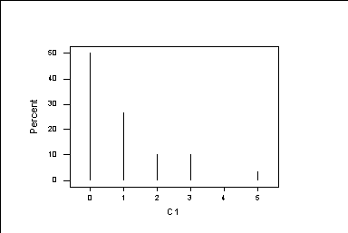
C1 COUNT CUMCNT PERCENT CUMPCT
0 15 15 50.00 50.00
1 8 23 26.67 76.67
2 3 26 10.00 86.67
3 3 29 10.00 96.67
5 1 30 3.33 100.00
N= 30
the columns are counts, cumulative counts, percent, cumulative percents.
Alternatively, we can do
MTB > tally c1;
SUBC> counts;
SUBC> percen;
SUBC> cumcounts;
SUBC> cumpercents.
To graph the percents we do,
MTB > Histogram C1;
SUBC> Percent;
SUBC> MidPoint;
SUBC> Project.
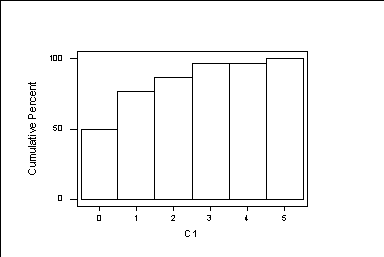
 To graph the cumulative percentages, we do:
MTB > Histogram C1;
SUBC> Cumulative;
SUBC> Percent;
SUBC> MidPoint;
SUBC> Bar.
To graph the cumulative percentages, we do:
MTB > Histogram C1;
SUBC> Cumulative;
SUBC> Percent;
SUBC> MidPoint;
SUBC> Bar.
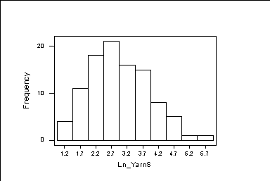
Next, we work with the yarn strength data: YARNSTRG.DAT, which is Example 2.7.
So, either we open the worksheet with this data or we enter this data.
We can get the Table 2.4 on frequencies in different interval by coding the data:
MTB > code (.95:1.45)1 (1.45:1.95)2 (1.95:2.45)3 (2.45:2.95)4 (2.95:3.45)5 &
CONT> (3.45:3.95)6 (3.95:4.45)7 (4.45:4.95)8 (4.95:5.45)9 (5.45:5.95)10 c1 c2
MTB > tally c2;
SUBC> all.
C2 COUNT CUMCNT PERCENT CUMPCT
1 4 4 4.00 4.00
2 11 15 11.00 15.00
3 18 33 18.00 33.00
4 21 54 21.00 54.00
5 16 70 16.00 70.00
6 15 85 15.00 85.00
7 8 93 8.00 93.00
8 5 98 5.00 98.00
9 1 99 1.00 99.00
10 1 100 1.00 100.00
N= 100
We can the histograms as follows
MTB > Set c3
DATA> 1.2 : 5.7 / .5
DATA> end
MTB > hist c1;
SUBC> midp c3;
SUBC> bar.
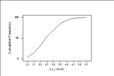
MTB > hist c1;
SUBC> midp c3;
SUBC> cumu;
SUBC> freq;
SUBC> conn.
******************
We can find the quartiles of the yarn strength data doing
MTB > descr c1
N MEAN MEDIAN TRMEAN STDEV SEMEAN
Ln_YarnS 100 2.9238 2.8331 2.8982 0.9378 0.0938
MIN MAX Q1 Q3
Ln_YarnS 1.1514 5.7978 2.2789 3.5732
We get:
MINIMUM Q1 MEDIAN Q3 MAX
1.1514 2.2789 2.8331 3.5732 5.7978
******************
To find the skewness and kurtosis of the yarn strength data we do:
MTB > let k1=std(c1)
MTB > let k2=mean((c1-mean(c1))**3)
MTB > let k3=k2/(k1**3)
MTB > print k3
K3 0.404016
MTB > let k4=mean((c1-mean(c1))**4)
MTB > let k5=k4/(k1**4)
MTB > print k5
K5 2.87466
We get that the skewness is 0.404016 and the kurtosis is 2.87466.
