Section 2.6.
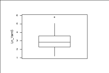
First we use the yarn strength data. We find the boxplot of these data
MTB > Retrieve  'A:\YARNSTRG.MTW'.
Retrieving worksheet from file: A:\YARNSTRG.MTW
**************************************
A boxplot consists of a box, whiskers, and outliers. A line is drawn across
the box at the median. By default, the bottom of the box is at the first
quartile (Q1), and the top is at the third quartile (Q3) value. The whiskers
are the lines that extend from the top and bottom of the box to the adjacent
values. The adjacent values are the lowest and highest observations that are
still inside the region defined by the following limits:

      Lower Limit:   Q1 - 1.5 (Q3 - Q1)
      Upper Limit:   Q3 + 1.5 (Q3 - Q1)

Outliers are points outside of the lower and upper limits and are plotted
with asterisks (*).
**************************************
MTB > boxplot c1


Using that
MTB > desc c1
                N     MEAN   MEDIAN   TRMEAN    STDEV   SEMEAN
Ln_YarnS      100   2.9238   2.8331   2.8982   0.9378   0.0938

              MIN      MAX       Q1       Q3
Ln_YarnS   1.1514   5.7978   2.2789   3.5732
We have that
Minimum=1.1514; Q1=2.2789; median=2.8331; Q3=3.5732; maximum=5.7978
In this case
Lower Limit:   Q1 - 1.5 (Q3 - Q1)= 2.2789-1.5(3.5732-2.2789)=0.8903
Upper Limit:   Q3 + 1.5 (Q3 - Q1)= 3.5732+1.5(3.5732-2.2789)=5.5146
The minimum is not an outlier, but the maximum is.
So, the lower whisker goes to the minimum. The upper whisker goes to
the biggest value in the data small than 5.5146. This value is  5.0904
Observe that
MTB > sort c1 c2
MTB > print c2


C2
  1.1514   1.1535   1.3436   1.4328   1.4570   1.5059   1.5219   1.5305
  1.6438   1.6787   1.7261   1.7837   1.7902   1.8926   1.8952   2.0813
  2.0968   2.1232   2.1306   2.1381   2.1771   2.2163   2.2364   2.2671
  2.2762   2.2872   2.3018   2.3459   2.3483   2.4016   2.4064   2.4190
  2.4240   2.4822   2.5000   2.5238   2.5264   2.5326   2.5364   2.5453
  2.5654   2.5724   2.5800   2.5813   2.6266   2.6537   2.6745   2.7243
  2.7317   2.8243   2.8418   2.8732   2.9382   2.9394   2.9908   3.0027
  3.0164   3.0693   3.0722   3.1166   3.1412   3.1860   3.1860   3.2108
  3.2177   3.2217   3.3077   3.3770   3.4002   3.4217   3.4603   3.4743
  3.4866   3.5017   3.5272   3.5886   3.6152   3.6162   3.6394   3.6398
  3.6561   3.7043   3.7071   3.7782   3.8849   3.9821   4.0017   4.0022
  4.0126   4.1251   4.3215   4.3389   4.4382   4.4563   4.5234   4.6315
  4.6426   4.8444   5.0904   5.7978

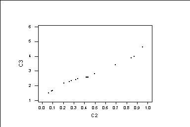
Next, we draw the quantile graph in page 37:
MTB > set c2
DATA> 1:100
DATA> end
MTB > let c2=c2/101
MTB > sort c1 c3
MTB > Plot C3*C2;
SUBC>   Symbol;
SUBC>     Type 5.


Next, we get the stem-and leaf- for the strength yard data
******************************************************************
A stem-and-leaf display shows the distribution of a variable in much the
same way as a histogram.  However, the initial digits of each value are
used to construct the display, so individual values can be read from the
display. A stem-and-leaf display has three parts:

   The first column shows a cumulative count of the number of values on that
line or on lines toward the nearer edge.  (The line that contains the median
shows a count of values on that line instead, enclosed in parentheses.)

   The second column of numbers holds the stems.

   The right-hand portion of the display holds the leaves.  Each leaf digit
represents an individual value.  The initial digits of that value are the
stem digits.  This is followed by the leaf digit.  Thus, a stem of 46 and a
leaf of 2 could represent the number 462, or 46.2, or .00462.  The position
of the decimal point is indicated by the UNIT of the leaf digit printed at
the top of the display.
**************************************************

MTB > stemandleaf c1

Stem-and-leaf of Ln_YarnS  N  = 100
Leaf Unit = 0.10


    5    1 11344
   15    1 5556677788
   34    2 0011112222233344444
  (21)   2 555555555566677888999
   45    3 000011112223344444
   27    3 5556666677789
   14    4 00013344
    6    4 5668
    2    5 0
    1    5 7
Next, we find robust statistics for location and dispersion.
To find the 5 % trimmed mean we do:
MTB > descr c1

                N     MEAN   MEDIAN   TRMEAN    STDEV   SEMEAN
Ln_YarnS      100   2.9238   2.8331   2.8982   0.9378   0.0938

              MIN      MAX       Q1       Q3
Ln_YarnS   1.1514   5.7978   2.2789   3.5732
The trimmed mean is 2.8982
Alternatively, we could do:
MTB > sort c1 c2
MTB > delete 1,2,3,4,5,96,97,98,99,100 c2
MTB > mean c2
   MEAN    =      2.8982
In this way, we can also find the 5 % trimmed standard deviation:
MTB > stdev c2
   ST.DEV. =     0.75951


