Section 3.1.



We work with the worksheet Place.mtw
MTB > Retrieve  'M:\PLACE.MTW'.
Retrieving worksheet from file: M:\PLACE.MTW
The data consists of the positions errors of 416 electronic components in 
26 printed circuits. c1 is the board number. c2 is the x deviation. c3 is 
the y-deviation. c4 is the angle deviation.

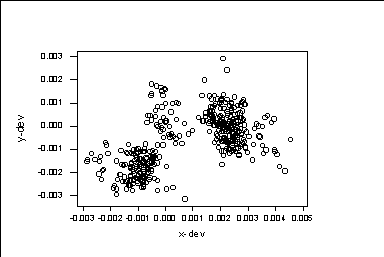
We can plot x-dev versus y-dev. The first variable goes to the y-axis and the
second variable goes to the x axis
MTB > plot c3*c2



This graph is in page 45 of the textbook. We see that there are clusters 
in the data.

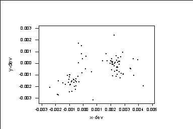
Instead of circles, we can use other symbols, for example, we get dots doing
MTB > plot c3*c2;
SUBC> symbol;
SUBC> type 5.



This is are different symbols you can get:
type 1 gives  o; type 2 gives +; type 3 gives x; type 4 gives *; 
type 5 gives .; type 'r' gives you that particular letter.
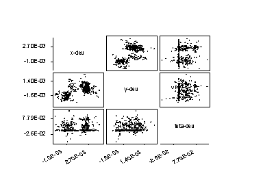
We can get plots for all combinations of variables by doing:
MTB > matrixplot c2 c3 c4

   

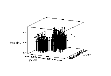
We can get 3 dimensional scatterplot of the 3 variables by doing:
MTB >  Pltx 'teta-dev'*'y-dev'*'x-dev';
SUBC> Symbol;
SUBC> project.

   

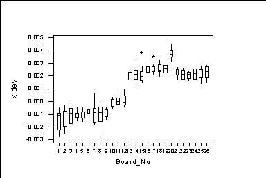
Next, we find the multiple boxplots of the x-dev against board number. 
We are getting a boxplot for all values in the data with the same board number:
MTB > boxplot c2*c1

   

Looking to this graph we conclude that there are 3 clusters:
1st one with the variables 1-9, 2nd one with the variables 10-12; 
3rd one with the variables 13-26. The observations corresponding to the 
1st cluster are the first 144. The observations corresponding to the 2nd 
cluster are the next 48. The observations corresponding to the 3rd cluster 
are the last 244. We can code this variables and do graphs where different 
"clusters" are graphed used different symbols:
MTB > set c5
DATA> 144(1) 48(2) 224(3)
DATA> end
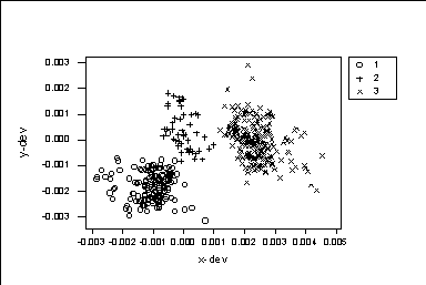
MTB > Plot 'y-dev'*'x-dev';
SUBC>   Symbol C5.



We see that certainly the three clusters of observations which we made, 
are behaving like 3 truly different clusters. All o's in the graph are in 
the lower left part of the graph. All +'s are in the middle. The x's are 
in the right.
Section 3.1.

Comments to: Miguel A. Arcones
