Section 3.4.
We work with the aluminum data in ALMPIN.mtw
MTB > Retrieve  'C:\MTBSEW\INDUST~1\MTW\ALMPIN.MTW'.

This data records of 6 dimension variables measured in mm of 70 aluminum
pins used in airplanes, in order of production. The six variables are
c2=diameter1, c3=diameter2, c4=diameter3, c5=cap diameter, c6=length of
the pin without cap, c7=length of the pin with cap. c2 c3 and c4 give
the pin diameter at three specified locations. c5 is the diameter of the
cap at the top of the pin. c6 and c7 are the length of the pin without
the cap and with the cap respectively.

First, we find the sample covariances and correlations of C2-c7
MTB > covariance c2-c7

               Diam1       Diam2       Diam3     CapDiam    Leng_NCP
Diam1     0.00026998
Diam2     0.00028323  0.00032441
Diam3     0.00025487  0.00028375  0.00027547
CapDiam   0.00029110  0.00031114  0.00028633  0.00036141
Leng_NCP -0.00016481 -0.00020445 -0.00014441 -0.00013789  0.00190693
Leng_WCP -0.00032568 -0.00040880 -0.00033282 -0.00032195  0.00154607

            Leng_WCP
Leng_WCP  0.00230697

MTB > corre c2-c7
          Diam1    Diam2    Diam3  CapDiam Leng_NCP
Diam2     0.957
Diam3     0.935    0.949
CapDiam   0.932    0.909    0.907
Leng_NCP -0.230   -0.260   -0.199   -0.166
Leng_WCP -0.413   -0.473   -0.417   -0.353    0.737

We should expect positive correlations between all the variables
(large pins are large in all the dimensions). However, this does not happen.
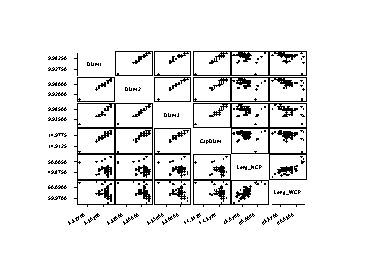
Some of the correlations are negative. We also can get multiple plots:
MTB > matrixplot c2-c7


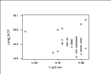
We see that some graphs show an isolated point. For example:
MTB > plot c6*c5


We have an isolated point on the left. We need to find the number of
the observation giving the smallest value.
MTB > rank c5 c15
MTB > print c15
MTB > set c16
DATA> 1:70
DATA> end
MTB > sort c16 c17;
SUBC> by c15.
MTB > print c16
66     2     3     9    13    14    17    18     1    15    16    20    21
22     7    19    23    24    25    43    45    57    68     4     5     6
8    10    11    12    26    27    29    30    31    33    34    35    38
39    41    42    46    48    51    54    58    59    60    62    63    65
70    28    32    36    37    40    44    50    52    53    55    56    61
64    67    69    47    49
In the column c15, we get the ranks of the observations.
In the column c17, we get the antiranks, the smallest c5 observation
is in Y(c17(1)); the second smallest c5 observation is in Y(c17(2));
and so on. In this way, we get that the isolated observation is the number 66.
The command: "sort c16 c17; by c15." orders the values of c16 in c17
according to the order in c15. In this way, we get that the isolated
observation is the number 66.
If we remove observation 66, we get bigger correlations
MTB > delete 66 c2-c7
MTB > corre c2-c7

          Diam1    Diam2    Diam3  CapDiam Leng_NCP
Diam2     0.923
Diam3     0.922    0.937
CapDiam   0.875    0.838    0.874
Leng_NCP -0.103   -0.150   -0.093   -0.019
Leng_WCP -0.313   -0.396   -0.328   -0.229    0.720

Next, we work with the solar cells data. The data consists of the
short circuit current of 16 solar cells measured in 3 different months.
MTB > Retrieve  'A:\SOCELL.MTW'.
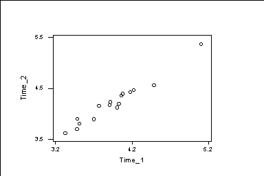
We try to find the linear relation between t1 and t2.
This is the graph of t1 and t2.
MTB > plot c2*c1


Next, we fit a regression line through this data:
MTB > regre c2 1 c1;
SUBC> resi c6;
SUBC> fits c7.

The regression equation is
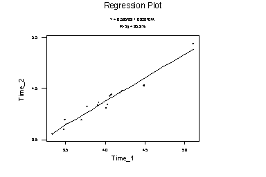
Time_2 = 0.536 + 0.929 Time_1

Predictor       Coef       Stdev    t-ratio        p
Constant      0.5358      0.2031       2.64    0.019
Time_1       0.92870     0.05106      18.19    0.000

s = 0.08709     R-sq = 95.9%     R-sq(adj) = 95.7%

Analysis of Variance

SOURCE       DF          SS          MS         F        p
Regression    1      2.5093      2.5093    330.84    0.000
Error        14      0.1062      0.0076
Total        15      2.6155

Unusual Observations
Obs.   Time_1     Time_2        Fit  Stdev.Fit   Residual    St.Resid
  9      5.11     5.3700     5.2814     0.0628     0.0886       1.47 X

X denotes an obs. whose X value gives it large influence.
************************************************************
We obtain the linear regression equation, a table of coefficients, an
estimate of standard deviation about the regression line, the coefficient
of determination (R-squared), R-squared adjusted for degrees of freedom,
the analysis of variance table, and unusual observations.
First, we get the least squares regression line y=a+bx, in this case:
               Time_2 = 0.536 + 0.929 Time_1
a is the constant term and b is the slope.
Then, we get columns related to the estimators a and b. The column
coefficients gives the estimates (a and b) of the linear equation. The
column Stdev gives estimates of the standard deviation of the coefficients.
This measure how precise our estimators are. In this case the estimation of
the constant term is not very precise, since Stdev=0.2031 and constant=0.5358.
But, the estimation of the slope is very precise:
b=0.92870 and its Stdev=0.05106

Next, we get the standard error s (the standard deviation of the residuals
around the regression line), the coefficient of determination R-sq and the
adjusted coefficient of determination R-sq(adj). R-sq measures the
proportion of variation which has been reduced by the regression.

Next, we get the analysis of variance table with degrees of freedom (df),
sums of squares (SS) and mean square errors (MS).
SOURCE       DF          SS          MS
Regression    1         SSR          MSR
Error        n-2        SSE          MSE
Total        n-1        SST

To find this table, we use the fits hat-y_i=a+bx_i
SSR=sum_i (hat-y_i - y-bar)^2
SSE=sum_i (y_i - hat-y_i)^2
SST=sum_i (y_i - y-bar)^2
We have that SST=SSR+SSE
The column mean square is obtained dividing the mean square error over
the degrees of freedom: MS=SS/df. MSR=SSR/1 MSE=SSE/(n-2). We have that
the MSE=0.0076=s^2=0.08709^2.

We have that the coefficient of determination R-sq=1-(SSE/SST)
Note that SSE/SST is the proportion of the variation (or sums of squares)
which is left after the regression. So, R-sq=1-(SSE/SST) is the proportion
of variation which is explained by the liner regression model.
We also have that R-sq=(correlation between X and Y)^2

Similarly, the adjusted coefficient of determination is
R-sq(adj)=1-(MSE/MST) is the proportion of the mean squares which is
left after the regression.

Finally, we get the observations which are either influential or outliers.
We could either X or XX for influential observations.
We could get either R or RR for outliers.
**********************
The subcommand
SUBC> resi c6;
put the residuals in the column c6.
The subcommand
SUBC> fits c7.
put the fits in the column c7.
**************************************************************************
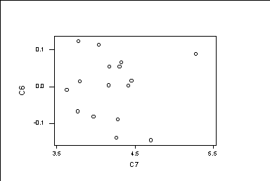
Next, we get the graph of residuals versus predicts.
MTB > plot c6 * c7


We should get a random graph. Values with a big residual are outliers.

The macro %Fitline graphs the pairs of observations and the regression line.
MTB > %Fitline 'Time_2' 'Time_1'
