Section 6.3.
A hypothesis testing has some similarities with the judicial system.
In the judicial system, we assume that the defendant is innocent,
unless it is proven guilty.
In a hypothesis testing problem, we assume that the null hypothesis
is true unless the data strongly support the alternative hypothesis.
In the judicial system, to conclude that the defendant is guilty, we
need to find characteristics of the perpetrator which match that of
the defendant and hold for a very small proportion of the population.
If we know the weight, blood type, race and other charateristics of
the perpetrator, these characteristics match the defendant and
they hold for one over a very small proportion (let us say one
over a million) of the people, then we conclude that the defendant is
guilty. It is almost impossible that by chance the defendant matches
the characteristic of the perpetrator by chance. It might happen by
chance that the supossedly innocent defendant
matches the characteristics of the perpetrator, but this is extremely
unlikable. In the other hand, if the characteristics of the suspect and
perpetrator which we match hold for a not so small proportion of the
peopple (let us say 10 %), then we do not have enough evidence to conclude
that the suspect is the perpetrator. It is possible by chance the
perpetrator and the suspect have those characteristic in common. So,
we reach a conclussion according to how likely is that the
matches between defendant and perpetrator occur by chance assuming
that the defendant is an innocent person from the general population.
In a hypothesis testing, we reject the null hypothesis, if the value
of the test statistic is very unlikely to appear assuming that the
null hypothesis is true. It might happen that by chance we get
that value of the statistic assuming the null hypothesis,
but this is extremely unlikable. In the other hand, if the value of
the test statistic is between the range of common values of the test
statistic, then we do not have enough evidence to reject Ho. So, we
either reject or accept Ho according to how likely is that the value
of the test statistic to appears.
The significance level alpha is the biggest value of the type I error. It is
the biggest probability for which we reject Ho assuming that Ho is true.
The significance level is how much evidence, we require to reject the
null hypothesis.The small alpha is, the more evidence we require to
reject Ho. If alpha=0.05, we asking for evidence in such a way, that
being Ho true 5 % of the times we make a mistake, because we get a
value of the statistic in the 5 % extreme values of the statistic.
The p-value of the test is the smallest significance level
for which we reject the null hypothesis. The p-value is the probability
that we get a value of the test statistic as extreme or more extreme than
the value from the data. The small the p-statistic is, the more
evidence we have to reject the null hypothesis.
For example, we test whether a coin is fair using 1000
throws of a coin. Suppose that we throw the coin 1000 times and
we get 560 heads. We test Ho:p=1/2 versus Ha:p /=1/2. Using minitab,
we can simulate 1000 throws of coin as many times as we want. Let us
simulate 2000 repeations of 100 throws of a coin:
MTB > random 2000 c1;
SUBC> bino 1000 .5.
MTB > desc c1
N MEAN MEDIAN TRMEAN STDEV SEMEAN
C1 2000 500.25 501.00 500.28 15.83 0.35
MIN MAX Q1 Q3
C1 443.00 554.00 489.00 511.00
MTB > histo c1
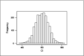
Looking to the simulations, we see that 560 is value very far off from the
values that we obtain when we throw a fair coin 1000. We almost never,
get a value as large as 560. The p-value of the test is 0.00000 and we
have a huge evidence to reject Ho.
If we do a test a the level .05, we reject Ho, when the number
of heads X, is either bigger than x(1-alpha/2) or smaller than x(alpha/2)
where P(Bino(1000,.5)= < x(.025))=.025
P(Bino(1000,.5)= < x(.975))=.975.
By the central limit theorem,
x(.025)=np-z(alpha/2)*sqrt(np(1-p))=500-1.96*15.8114=469.010
and
x(.975)=np-z(1-alpha/2)*sqrt(np(1-p))=500+1.96*15.8114=530.990
So, we reject Ho if either X=< 469 or X>=531
We have that approximately 95 % of our simulations fall between
470 and 530. 560 is outside the interval of reasonable outcomes.
So, we reject Ho.
***********************************************************
We can use minitab to do test for the mean of a normal distribution,
both knowing and not knowing the variance.
If we do not know the variance, we do a z-test.
For example, in the car data, assuming that sigma=3,
we can test Ho: mu=34 versus Ha: mu>34:
MTB > Retrieve 'C:\ISTAT\CAR.MTW'.
Retrieving worksheet from file: C:\ISTAT\CAR.MTW
MTB > ztest 35 3 c3;
SUBC> alte 1.
TEST OF MU = 35.000 VS MU G.T. 35.000
The assumed sigma = 3.00
|
N |
MEAN |
STDEV |
SE MEAN |
Z |
P VALUE |
| Tur_Diam |
109 |
35.514 |
3.321 |
0.287 |
1.79 |
0.037 |
We conclude that there is enough evidence at the level .05 to
reject Ho. The evidence is mild, not very strong.
So, we do:
MTB > ztest muo sigma variable
We are getting
that n=109, x-bar=35.514, s=3.321, sigma/sqrt(n)=0.287, and
z=sqrt(n)*(x-bar - muo)/sigma=1.79 and the p-value=0.037


By default, minitab do a two sided test. If we do not specify mu,
minitab takes mu=0 as default.
To do one sided tests, we use the subcommand alter
If ALTERNATIVE = -1 then mu < muo is used.
If ALTERNATIVE = 1, then mu > muo is used.
If we do not know the variance, we do a t-test:
MTB > ttest 35 c3;
SUBC> alte 1.
TEST OF MU = 35.000 VS MU G.T. 35.000
|
N |
MEAN |
STDEV |
SE MEAN |
T |
P VALUE |
| Tur_Diam |
109 |
35.514 |
3.321 |
0.318 |
1.62 |
0.055 |
We conclude that there is not enough evidence at the level .05
to reject H(o). mu could be 35.
We are getting that n=109, x-=35.514, s=3.321,
s/sqrt(n)=0.287, and t=(x--muo)/s/sqrt(n)=1.62
Note that in the z-test, we reject the null hypothesis and in
the t-test do not.
This happens because sigma=3 is smaller than s=3.321.
As small as sigma is as most likely we reject the null hypothesis.
