In this chapter, we only consider the two way layout without replications. We can do anova for a two way layout without replications. We also can apply the Friedman test. I run the following script file in the data in Table 7.1 (page 274) of the textbook.
****** program 7a **********
x_c(5.40,5.50,5.55,5.85,5.7,5.75,5.2,5.6,5.5,5.55,5.5,5.4,5.9,5.85,5.7,5.45,5.55,5.6,5.4,5.4,5.35,5.45,5.5,
+ 5.35,5.25,5.15,5.00,5.85,5.8,5.7,5.25,5.2,5.1,5.65,,5.55,5.45,5.6,5.35,5.45,5.05,5.,4.95,5.5,5.5,5.4,5.45,
+ 5.55,5.5,5.55,5.55,5.35,5.45,5.5,5.55,5.5,5.45,5.25,5.65,5.6,5.4,5.7,5.65,5.55,6.3,6.3,6.25)
n_22
k_3
q_7
N_10000
x.matrix_matrix(x,ncol=k,byrow=T)
block <- factor(as.vector(row(x.matrix)))
treatment <- factor(as.vector(col(x.matrix)))
print(mean(x))
print(median(x))
print(stdev(x))
print(apply(x.matrix,2,mean))
print(apply(x.matrix,2,stdev))
print(apply(x.matrix,2,median))

fnames_list(treatment=paste("treatment ",LETTERS[1:k]),block=paste("block ",1:n))
design_fac.design(c(k,n),fnames)
two.layout_data.frame(design,x)
print(two.layout)

mini_min(x)
maxi_max(x)
plot(treatment,x,ylim=c(mini,maxi))
par(mfrow=c(1,4),cex=1.2)
boxplot(x,ylim=c(mini,maxi))
boxplot(x.matrix[,1],ylim=c(mini,maxi))
boxplot(x.matrix[,2],ylim=c(mini,maxi))
boxplot(x.matrix[,3],ylim=c(mini,maxi))

print(aov(x~block + treatment,two.layout))
print(summary(aov(x~block + treatment,two.layout)))
r_c(0,0,0)
ra_rep(0,n*k)
ranks_matrix(ra,ncol=k,byrow=T)
rep_matrix(ra,ncol=k,byrow=T)
for(i in 1:n){
r_r+rank(x.matrix[i,])
ranks[i,]_rank(x.matrix[i,])
for(j in 1:k){
rep[i,j]_ rle(sort(ranks[i,]))$lengths[j]
if (is.na(rep[i,j])) rep[i,j]_0
}
}
print(ranks)
print(rep)
print(friedman.test(x.matrix, treatment,block))
correc_(sum(rep^3)-(n*k))/(k-1)
friedman_12*(sum((r-(n*(k+1)/2))^2))/(n*k*(k+1)-correc)
print(friedman)
p.value_1-pchisq(friedman,df=k-1)
print(p.value)

friedman.sim_rep(0,N)
ranks.sim_rep(0,k)
for(p in 1:N){
r_c(0,0,0)
for(i in 1:n){
ranks.sim_sample(ranks[i,], size=k, replace=F)
r_r+ranks.sim
}
friedman.sim[p]_12*(sum((r-n*(k+1)/2)^2))/(n*k*(k+1)-correc)
}
p.value.sim_sum(friedman.sim>friedman)/N
print(p.value.sim)
Next, we see the outcome of the previous script file. We can look to the means and medians, overall and by treatment.
> print(mean(x))
[1] 5.512121
> print(median(x))
[1] 5.5
> print(stdev(x))
[1] 0.2667555
> print(apply(x.matrix, 2, mean))
[1] 5.543182 5.534091 5.459091
> print(apply(x.matrix, 2, stdev))
[1] 0.2718085 0.2597555 0.2728319
> print(apply(x.matrix, 2, median))
[1] 5.500 5.525 5.450
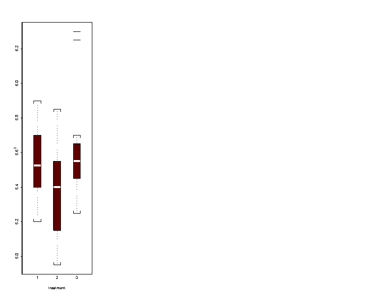
Looking to the means, the second treatment seems to be the smallest. But, looking to the medians, the second treatment seems to be the biggest. The standard deviation is 0.2667555. The differences between the different means do not seems to significant.
Here are the graphs.


Note that we have aparticular structure of the data, all previous indications do not use the the structure of the data. Previously, we have combined all data for one treatment in one block. The data does not consist of three blocks.
This is the outcome of the anova:
 > print(aov(x ~ block + treatment, two.layout))
Call:
   aov(formula = x ~ block + treatment, data = two.layout)

Terms:
                   block treatment Residuals
 Sum of Squares 4.218636  0.093712  0.312955
Deg. of Freedom       21         2        42

Residual standard error: 0.08632091
Estimated effects are balanced
> print(summary(aov(x ~ block + treatment, two.layout)))
          Df Sum of Sq   Mean Sq  F Value       Pr(F)
    block 21  4.218636 0.2008874 26.96006 0.000000000
treatment  2  0.093712 0.0468561  6.28831 0.004084101
Residuals 42  0.312955 0.0074513
The p-value of the anova test is 0.004084101.
So, we reject the null hypothesis at the level 5 %. Given the small sample size, we cannot assume normality of the data. A more realistic approach is to use a nonparametric test. We do the Friedman test:
> print(friedman.test(x.matrix, treatment, block))

	Friedman rank sum test

data:  x.matrix and treatment and block
Friedman chi-square = 11.1429, df = 2, p-value = 0.0038
alternative hypothesis: two.sided

> print(friedman)
[1] 11.14286
> p.value <- 1 - pchisq(friedman, df = k - 1)
> print(p.value)
[1] 0.003805041
The value of the Friedman statistic is 11.14286. The p-value of the Friedman test is 0.003805041 We reject the null hypothesis.
We also can estimate the p-value of the Friedman test using simulations. The outcome of the simulations is
> print(p.value.sim)
[1] 0.0033
We get a p-value very close to the p-value using the chisquare approximation.
