Subsampling Winner Algorithm for Variable Selection in the Classification Setting
This algorithm conducts variable selection in the classification setting. It repeatedly subsamples variables and runs linear discriminant analysis (LDA) on the subsampled variables. Variables are scored based on the AUC and the t-statistics. Variables then enter a competition and the semi-finalist variables will be evaluated in a final round of LDA classification. The algorithm then outputs a list of variable selected.
Table of Content
Software swa
How to install the R package swa, swa()
How to run swa()
Details of the algorithm
1. Software nFCA
The swa package includes a main R code swa(). It takes in the design matrix and the response as inputs and outputs a list of selected variables and a final multiple linear regression model using the selected variables.
2. How to install, load and unload the package swa in R
  > install.packages("swa")   # install swa package
  > library(swa)    # load swa package
  > detach(package:swa)    # unload swa package
You may also first download the package to your computer and install locally.
> install.packages("swa_0.8.1.tar.gz", repos = NULL, type = "source")
3. How to run swa in R
Upload and get help:
  > library(swa)
  > ?swa
Consider a simple example below.
  > set.seed(1)
  > x <- matrix(rnorm(20*100), ncol=20)
  > b = c(0.5,1,1.5,2,3);
  > y <- x[,1:5]%*%b + rnorm(100)
  > y <- as.numeric(y<0)
  > X <- t(x)
  > swa(X,y,c(3,5,10,15,20),5,500,MPplot = TRUE) ;
In this example, the design is a 100 by 20 matrix with 20 independent variables. Only the first five independent variables bear true signals that influence the response. Variable 5 has a strong signal while variable 1 has a weak signal. When the MPplot option is set on, then a multi-panel plot is produced.
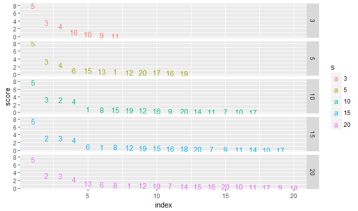 |
The MP plots show that the upper arm sets, i.e., the points above the elbow point of each panel plot, started to be stabilized at s = 10. Thus, we fix s = 10 below.
> sum_swa <- swa(X,y,10,5,500)
> sum_swa
$index
[1] 5 3 2 4 1

$summary

Call:
lm(formula = yy ~ ., data = dataXY)

Residuals:
     Min       1Q   Median       3Q      Max
-2.98810 -1.06555 -0.02721  1.17308  2.29243

Coefficients:
            Estimate Std. Error t value Pr(>|t|)
(Intercept)   0.1927     0.1394   1.382 0.170266
X5           -0.9973     0.1238  -8.058 2.42e-12 ***
X3           -0.4877     0.1265  -3.854 0.000212 ***
X2           -0.4290     0.1265  -3.391 0.001019 **
X4           -0.4216     0.1371  -3.074 0.002763 **
X1           -0.1090     0.1356  -0.804 0.423531
---
Signif. codes:  0 ‘***’ 0.001 ‘**’ 0.01 ‘*’ 0.05 ‘.’ 0.1 ‘ ’ 1

Residual standard error: 1.375 on 94 degrees of freedom
Multiple R-squared:  0.5559,	Adjusted R-squared:  0.5323
F-statistic: 23.54 on 5 and 94 DF,  p-value: 2.885e-15


$step_sum

Call:
lm(formula = yy ~ X5 + X3 + X2 + X4, data = dataXY)

Residuals:
     Min       1Q   Median       3Q      Max
-2.92167 -1.13646  0.03455  1.22929  2.29080

Coefficients:
            Estimate Std. Error t value Pr(>|t|)
(Intercept)   0.1942     0.1391   1.396 0.165992
X5           -1.0122     0.1221  -8.287 7.47e-13 ***
X3           -0.4897     0.1263  -3.878 0.000194 ***
X2           -0.4266     0.1262  -3.379 0.001055 **
X4           -0.4152     0.1366  -3.039 0.003070 **
---
Signif. codes:  0 ‘***’ 0.001 ‘**’ 0.01 ‘*’ 0.05 ‘.’ 0.1 ‘ ’ 1

Residual standard error: 1.372 on 95 degrees of freedom
Multiple R-squared:  0.5529,	Adjusted R-squared:  0.5341
F-statistic: 29.37 on 4 and 95 DF,  p-value: 6.774e-16
The final model perfectly recovers the five true variables. The stepwise selection removes X1, which has the weakest signal (hence is not expected to be recovered.) We next check the results with a larger m = 1000.
> sum_swa <- swa(X,y,10,5,1000)
> sum_swa
$index
[1] 5 3 2 4 6

$summary

Call:
lm(formula = yy ~ ., data = dataXY)

Residuals:
     Min       1Q   Median       3Q      Max
-2.85483 -1.06089 -0.00216  1.19698  2.40598

Coefficients:
            Estimate Std. Error t value Pr(>|t|)
(Intercept)   0.1904     0.1391   1.369 0.174247
X5           -1.0010     0.1225  -8.172 1.39e-12 ***
X3           -0.4856     0.1262  -3.847 0.000218 ***
X2           -0.4245     0.1261  -3.365 0.001109 **
X4           -0.4016     0.1371  -2.929 0.004271 **
X6            0.1574     0.1459   1.079 0.283566
---
Signif. codes:  0 ‘***’ 0.001 ‘**’ 0.01 ‘*’ 0.05 ‘.’ 0.1 ‘ ’ 1

Residual standard error: 1.371 on 94 degrees of freedom
Multiple R-squared:  0.5583,	Adjusted R-squared:  0.5349
F-statistic: 23.77 on 5 and 94 DF,  p-value: 2.247e-15


$step_sum

Call:
lm(formula = yy ~ X5 + X3 + X2 + X4, data = dataXY)

Residuals:
     Min       1Q   Median       3Q      Max
-2.92167 -1.13646  0.03455  1.22929  2.29080

Coefficients:
            Estimate Std. Error t value Pr(>|t|)
(Intercept)   0.1942     0.1391   1.396 0.165992
X5           -1.0122     0.1221  -8.287 7.47e-13 ***
X3           -0.4897     0.1263  -3.878 0.000194 ***
X2           -0.4266     0.1262  -3.379 0.001055 **
X4           -0.4152     0.1366  -3.039 0.003070 **
---
Signif. codes:  0 ‘***’ 0.001 ‘**’ 0.01 ‘*’ 0.05 ‘.’ 0.1 ‘ ’ 1

Residual standard error: 1.372 on 95 degrees of freedom
Multiple R-squared:  0.5529,	Adjusted R-squared:  0.5341
F-statistic: 29.37 on 4 and 95 DF,  p-value: 6.774e-16
It now captured X2,X3,X4,X5, and also a noise variable X6 that is not as significant as the former 4 covariates X2-X4.
4. Details of the algorithm
Let \(d\) be the (total) dimension and \(d_0\) be the number of true variables. We let \(m\) be the number of subsamplings, \(s\) be the sampling size, \(q\) be both the number of subsamplings to keep, and the number of semifinalist variables.
For \(t=1:m\)
Subsample a subset of \(s\) variables, \(\mathcal{S}_t\), from the \(d\) variables with absolute marginal \(t\)-statistic greater than \(\alpha=0.001\).
Run LDA on the data \((\mathbf{X}_{\mathcal{S}_t},\mathbf{y}_{\mathcal{S}_t})\) which yields the area under the ROC curve (AUC-ROC) \(U_t\) and \(t\)-statistic \(T_{t,i}\) for each variable \(i\in\mathcal{S}_t\).
Keep the best \(q\) subsampled sets with the highest AUC-ROC \(U_t\). Let \(\mathcal{T}\) be the index set of these subsamples.
For each variable \(i\), calculate its average absolute value of the \(t\)-statistic, reweighted by the square root of the AUC-ROC value of the set, \(r_i = {\sum_{t\in\mathcal{T}} 1[i\in \mathcal{S}_t]}^{-1} \sum_{t\in\mathcal{T}} U_t^{1/2}|T_{t,i}|\).
Let \(\mathcal{Q}\) be the index set of the variables with the \(q\) highest \(r_i.\)
Run LDA on the data \((\mathbf{X}_{\mathcal{Q}},\mathbf{y}_{\mathcal{Q}})\). For each variable \(i\in\mathcal{Q}\), the \(p\)-value is adjusted using a multiple comparison method such as the Bonferroni method or the Benjamini-Hochberg procedure.